Chapter 6 Giving your suppliers orders and future guidance

Figure 6.1: This chapter is currently under construction, it will probably be ready in week 8 or 9 of the semester. Please come back later
Map of the chapter is required here
The final stage of the planning cycle is to issue call-off and forecasted orders to your suppliers. The call-off orders are instructions to your supplier about what to deliver in the current period. The forecast orders are guidance, a prediction but not a guarantee, of the requirements in the future. The call-off and order forecasts can be issued by your ERP system, although some companies do this via fax, EDI or email. Planned forecasted orders for the MRP module can come from either the Planning module or the Scheduling module. The purchasing department maintains lead-time information in the MRP module. Q. How do they know it is correct? It is important, to get at least the average lead-time right, even if you have a stochastic lead-time. Often companies presume that erring on the side of caution and high-balling the lead-time is the best option but this result in excess inventory. Perhaps the logistics department should be informing the purchasing department what the actual lead-times are (monitor them and report deviances.) these are ideas that need to be addressed
Some suppliers may be under a VMI contract to supply your factory. Here no safety stock is maintained in the MRP system, but current inventory levels and order forecasts may be passed to the supplier so that they may infer recent usage from the net change in inventory levels as well as giving them guidance for long-term capacity planning. VMI suppliers may be delivering to an open purchase order with a large quantity and no financial information. Otherwise, the receiving dock may turn away the undocumented supply. Suppliers on a regular supply chain contract by given firm call-off orders and a purchase-order each period and guidance on future orders. Items brought from a spot market may still require an MRP process to exist, if only for your long term financial planning activities.
6.1 The bill of materials.
BOM is also known as a Production Process Module, Product Data Structure.
Figure 38. An example BOM (Perhaps an IKEA product?)
The BOM infomration in your MRP system needs to be correct. Over time, engineering changes will be made to the product as components are modified and recipes improved. This whole engineering change process requires careful management. Quality losses, scrap, and yield rates need to be monitored and your MRP system updated with the latest information. Lead-times may change when parts are sourced from different vendors. Suppliers may move the location of their production activities or use different transportation lanes.
It is critical to use the correct units of measurements in the MRP system. For example, some countries still use pounds and ounces for weight instead of kilograms or feet and inches instead of meters and centimeters. A British ton (or long ton) is 1016.047kg, the U.S. ton (or short ton) is 907.1847kg, and a metric ton (or tonne) is a 1000kg. The imperial gallon is 4546cc. The U.S. liquid gallon is 3785.41cc or approximately 3.785cc. The U.S. dry gallon is 4405cc.
Dependent demand, independent demand
Supplier lot sizes, Lot for lot
6.2 MRP nervousness
Explain what MRP nervousness problem in here.
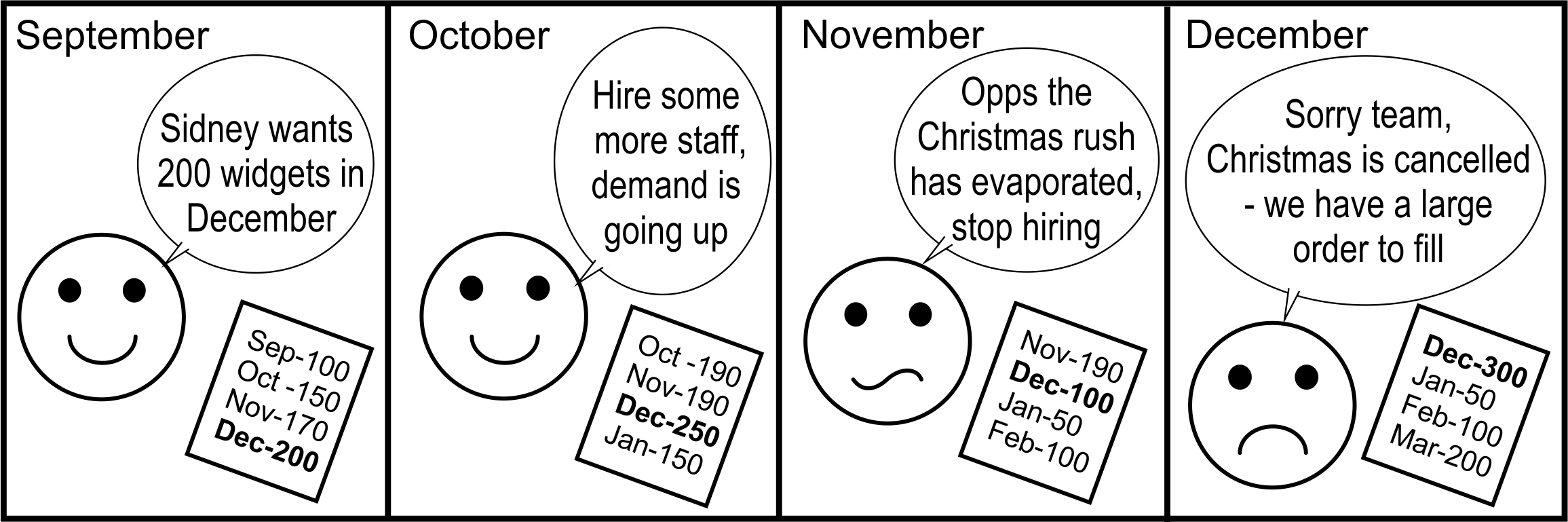
Figure 6.2: MRP nervousness: Rescheduling the schedules you just rescheduled
Quantity Demand forecast for delivery in week
Table 33. Example MRP data (Call-off orders in bold)
| First Header | Second Header | Third Header |
|---|---|---|
| Content | Long Cell | |
| Content | Cell | Cell |
| New section | More | Data |
| And more | With an escaped ‘|’ |
The demand experienced by the supplier each week (the call-off orders) is highlighted in bold in Table 33. The variance of the supplier’s demand is part of the Bullwhip calculation, and we find them as the bold numbers lying on the diagonal in Table 33. The supplier’s demand was 120 in week 0, 80 in the week -1 , 90 in the week -2, 110 in the week -4 and 100 in the week -5 and so on. Demand fluctuates from week to week. We can also see another form of uncertainty in Table 33. The forecasts of the call-off orders made in previous weeks were both inaccurate and are also variable from week to week. For example, in week -1, the forecast of the supplier’s demand in week 0 was 101. However, when week 0 comes along, the actual call-off order was only 120. The forecast of the demand in the week -1, made in the week -2, was 122; the forecast made in the week -2 was 103. This type of forecast uncertainty is an effect known as MRP nervousness. The numbers here need to be carefully checked.
Table 34. Example calculation of the MRP nervousness measure with Exponential Smoothing forecasts
Suppliers would like to have accurate predictions of future demand so that they may set-up their supply chain to meet future demand. This may mean ordering raw materials, hiring staff, installing production capacity (machines, etc.) as well as producing the quantity required. If the forecast is too high, then perhaps the supplier has ordered too much raw material, made too much product, or hired too many staff, etc. If the forecasts are too low, perhaps the supplier did not order enough raw material or must work overtime with the smaller than required workforce he has in place. We can see then that it is just not the variability of the amount of work that has to be done; the predictability of the work required is also important.
To manage this MRP nervousness effect, we need a measure of the nervousness. We do this by first calculating the variance of the j-step ahead order forecast error with
\[\begin{align} \Delta[j]=\lim_{T\to\infty}\left( \frac{1}{T}\sum_{i=0}^T \left( \hat{O}_{t-j-i,t-i}-O_{t-i} \right)^2 \right) \end{align}\]
Imagine it is now time \(t=0\) in Table 33 with \(j=1\), the one period ahead order forecast error is given by
\[\begin{equation} \Delta[1]=\frac{1}{5}\left((82-120)^2+(122-80)^2+(120-90)^2+(112-110)^2+(102-100)^2\right)=672 \end{equation}\]
As a forecast error in the near future is likely to be more costly than one in the distant future, and as a large forecast error is more expensive than a small error, an exponentially weighted sum of order forecast error variances is a natural measure of nervousness:
Here the exponential weighting factor, \(w\), determines how quickly the variability of the future order forecast errors decay away (in much the same way as the forecasting parameter in exponential smoothing behaves). When \(w\) is large, the influence of the forecast error decays away more quickly than when \(w\) is small. When \(0<w<1\), the sum in (22) converges to a finite number, allowing us to measure the nervousness produced by different replenishment system designs. Lower \(\Delta\) indicate more accurate future guidance (that is, less nervousness is created), and the easier it will be for your suppliers to organize their activities to meet demand.
| j | \(\Delta[j]\) | \(w(1-w)^{j-1}\) | \(w(1-w)^{j-1}\Delta[j]\) |
|---|---|---|---|
| 1 | 561 | 0.5 | 280.5 |
| 2 | 672 | 0.25 | 168 |
| 3 | 689 | 0.125 | 86.125 |
| 4 | 696 | 0.0625 | 43.5 |
| 5 | 705 | 0.03125 | 22.03125 |
| 7 | 748 | 0.015625 | 11.6875 |
| Total | \(\Delta=611.84\) |
What about bias and gaming? Bias in the order forecasts is also important. If the future guidance is based on the planning book forecasts, and the manual interventions in the forecasts are minimal the bias in the MRP order forecast should be minimal. People have a tenancy to communicate an inflated forecast to a) secure supply by tricking the supplier to invest in extra capacity, b) improve their position in pricing negotiations.
OUT policy uses the forecasts from the forecasting system POUT policy can use the PFG mechanism
\[\begin{equation} \hat{o}_{t,t+j}=\hat{d}_{t,t+T_s+1+j}+\frac{1}{T_i}\left(\frac{T_i-1}{T_i}\right)^j \left( TNS-ns_t+\sum_{i=1}^{T_s}\left(\hat{d}_{t,t+1}-o_{t-1}\right)\right) \end{equation}\]
Month versus weeks, long versus short Capacity limited
The cost of the MRP nervousness
- Add some typical cosst in here
- and soem more costs
- Demands greater then the forecasts within the lead-time result in lower inventory, potentially shortages
- Increase
A VMI supplier, who has a stock of product in your goods in the warehouse will be able to satisfy your demand within the next week, i.e. . The source of the data for the VMI supplier call-off order is the detailed schedule. The VMI supplier will also be given a set of order forecasts, one for each week (or month if they wish to have monthly data) into the future. A non-VMI supplier, however, many have to make, but will definitely have to ship to your factory will probably not be able to deliver your requirements with the current planning cycle, **** this does not make sense *** i.e. . In this case, the supplier’s firm order and the forecasted order will be based on future forecasts that have come from the planning book. See Table 36, where we have assumed the non-VMI supplier’s lead time is
Table 36. Source of the data in the MRP information given to suppliers
It is easy to appreciate that in the VMI case that we do not have to hold a safety stock of raw materials, as the supplier can deliver the product with zero lead-time, based on our actual usage. However, the non-VMI supplier case, the supplier delivers to a forecast of future demand; we bear the inventory risk if our forecast is incorrect. Thus in the non-VMI case, our safety stock must cover at least the variability of the forecasts errors (as well as the ability of the supplier to deliver the correct quantity, on-time and at the right quality standard.
Need a high-level map of the workflow in the MRP task. Perhaps based on Don’s map. If you are only concerned with your inventory costs, then you should use OUT/MMSE If your main concern is capacity costs in the supplier then POUT/MMSE If your main concern is inventory cost in the supply chain the use the POUT/PFG.
Measuring supplier performance Quality issues, On time in full deliveries, lead-time, inventory
6.2.1 ERP implementation issues
Clean your MRP data. This gives you a great opportunity to have correct, consistent supply chain data from which you can base decisions. Part numbers…. Is the production counted only once? For example, if independent demand is coming from the Detailed Scheduling module, has that independent demand also been removed from the Planning book or is it counted twice. Dependent demand. Coming from the demand from independent demand, through the bill of materials. How far down the BOM do you explode the BOM?
Data integrity (check to see if all these were considered in the forecast chapter) What consists of a good point to measure/record demand? When are items removed from inventory? When production completions are back-flushed in the MRP system to claim the raw materials? Transactions need to be completed in a uniform manner at all times and in all parts of the company. Without good data you are blind.
Notes. Suppliers- VMI or non-VMI. Talk to them, what information do they require? In what format/buckets, how is it delivered? Passing around spreadsheets, faxes, EDI, integrated ERP systems?
Factors to communicate with your suppliers:
Major turning points in demand
Design changes
End of product life cycle/all-time builds
Holiday and shutdowns
Feedback quality issues, quality holds, quarantines and on-holds
Missing products/over-deliveries
VMI inventory levels
Packaging returns
Need an MRP table in here somewhere based loosely on the MRP table in Lexmark. And explain it.
Weekending Month
1 July 7 July 14 July 21 July 28 July Aug Sept Oct
Inventory 300
Actual Usage 100
Planned Usage 90 100 100 100 400 400 400
Table 37. Example MRP information passed to a VMI supplier on 7th July 2016
Month PO Number Current open order quantity Due date requested Alterations to previous requests Out months quantities
July Xxxx 7560 7 July
Aug X 6120 7 Aug
Sept X 6480 7 Sept
Oct 5760
Nov 8100
Table 38. Example MRP information passed to a non-VMI supplier on 7th July 2016 (Ts here is 3 months) Spread out the deliveries over the month to smooth the workload at goods-in. Schedule the high-value items to be received at the beginning of the month (then at the end of the month, production would have consumed that inventory, make the inventory cost figures look good.